Michaelis-Menten (v vs [S]): use when Km and Vmax are already known and you want velocity at a specific [S], or an intuitive picture of saturation.
Lineweaver-Burk (1/v vs 1/[S]): use when you have raw data and need Km/Vmax by hand, the reciprocal transform turns the hyperbola into a line, or when you need to diagnose inhibition type from how the line changes.
Same equation, two plots
Both come from the same starting point: v = Vmax[S] / (Km + [S]). Plotted directly, that's a hyperbola. It rises steeply at low [S], then bends over and creeps toward Vmax without ever quite reaching it. That shape is intuitive to look at but painful to fit by hand: Vmax is an asymptote, not a point on the curve, so estimating it by eye is guesswork.
Take the reciprocal of both sides and rearrange, and the same relationship becomes a straight line: 1/v = (Km/Vmax)(1/[S]) + 1/Vmax. Now Vmax and Km are just the intercept and slope of a line, solvable with ordinary linear regression, which is exactly why Lineweaver-Burk exists: it was invented so Michaelis-Menten kinetics could be fit before anyone had a computer to run nonlinear regression.
Worked example: the same 6 data points, both ways
Enzyme velocity measured at 6 substrate concentrations:
| [S] | v | 1/[S] | 1/v |
|---|---|---|---|
| 0.5 | 21 | 2.000 | 0.0476 |
| 1 | 34 | 1.000 | 0.0294 |
| 2 | 49 | 0.500 | 0.0204 |
| 4 | 67 | 0.250 | 0.0149 |
| 8 | 79 | 0.125 | 0.0127 |
| 16 | 90 | 0.0625 | 0.0111 |
Plotted as v vs [S] directly, this is visibly curving toward some asymptote somewhere above 90, but where, exactly? Hard to say by eye. Plotted as 1/v vs 1/[S] instead, it's a straight line, and an ordinary linear regression solves it exactly:
The other reason to use Lineweaver-Burk: diagnosing inhibition
Beyond fitting raw data, Lineweaver-Burk earns its place because the three classic inhibition types are far easier to tell apart on a straight line than on a curve. Each type of inhibition changes the line's slope and intercepts in a specific, recognizable way.
Worked example: same inhibitor concentration, two different mechanisms
Baseline enzyme: Vmax = 100 µM/min, Km = 25 µM. Inhibitor present at a concentration equal to Ki (so the ratio r = [I]/Ki = 1) in both cases, only the inhibition type differs.
| Km(app) | Vmax(app) | LB slope | LB y-int | LB x-int | |
|---|---|---|---|---|---|
| No inhibitor | 25.0 | 100.0 | 0.250 | 0.0100 | −0.040 |
| Competitive | 50.0 | 100.0 | 0.500 | 0.0100 | −0.020 |
| Noncompetitive | 25.0 | 50.0 | 0.500 | 0.0200 | −0.040 |
Competitive inhibition keeps the exact same y-intercept as the baseline (0.0100 both times). That shared intercept is the signature of competitive inhibition on sight. Noncompetitive inhibition instead keeps the exact same x-intercept (−0.040 both times), which is its signature instead. Both of those matches are easy to spot on a straight-line plot and essentially impossible to eyeball on the raw curved Michaelis-Menten plot.
See these lines drawn live in the enzyme kinetics simulator →When to use each, at a glance
| Situation | Use |
|---|---|
| You have raw (v, [S]) data and need Km/Vmax by hand | Lineweaver-Burk |
| You need to diagnose competitive vs. noncompetitive vs. uncompetitive inhibition | Lineweaver-Burk |
| You already know Km/Vmax and want v at a specific [S] | Michaelis-Menten |
| You want an intuitive picture of saturation kinetics | Michaelis-Menten |
| You're fitting real lab data with software, for publication | Neither by hand, nonlinear regression directly on the curve |
Common mistakes
Trusting Lineweaver-Burk as "more accurate." It's the opposite for precise work, taking reciprocals amplifies the relative error of low-velocity (low [S]) points, since small errors in small numbers become large errors once inverted. It's the standard teaching method because it's solvable by hand, not because it's statistically ideal.
Trying to read Vmax straight off a Michaelis-Menten plot. It's an asymptote the curve approaches but never reaches, eyeballing it is imprecise even with a well-drawn curve.
Comparing the wrong intercept. Competitive inhibition is diagnosed by a shared y-intercept; noncompetitive by a shared x-intercept. Mixing these up is the single most common Lineweaver-Burk mistake on exams.
Practice problem
1. An enzyme has Vmax = 100 µM/min and Km = 25 µM. Under uncompetitive inhibition with [I] = 100 µM and Ki = 50 µM (so r = 2), find the Lineweaver-Burk slope, y-intercept, and x-intercept, and compare each to the uninhibited baseline.
Show answer
Related tools: Michaelis-Menten fitter · Enzyme kinetics simulator · all biochem tools. More MCAT explainers: the 3 MCAT buffer question types · how to calculate pI without a calculator.
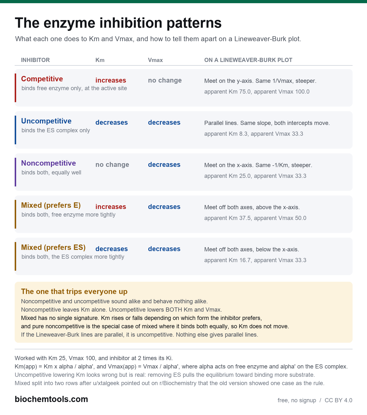
Printable inhibition chart
All four inhibition patterns on one page: what each does to Km and Vmax, how it binds, and the shape it makes on a Lineweaver-Burk plot.

Download the chart, or the print-friendly white version. Free for a study guide or class handout, no attribution needed. See all the printable charts. Every arrow on it is computed from the same alpha and alpha-prime equations this page uses, so the chart and the worked examples cannot disagree.
FAQ
Is Lineweaver-Burk more accurate than fitting the curve directly?
No, less accurate for precise work. Reciprocals amplify the relative error of low-velocity points, giving them disproportionate weight in the regression. Software fits the untransformed hyperbola directly for publication-quality numbers; Lineweaver-Burk remains standard in coursework because it's solvable by hand.
Can I read Vmax directly off a Michaelis-Menten plot?
Only approximately. It's the asymptote the curve approaches but never reaches, so eyeballing it is imprecise even with a well-drawn curve. This is a major reason the linearized approach is preferred whenever you need an actual number.
Why are inhibition types easier to tell apart on Lineweaver-Burk?
On the raw curve, different inhibition types can look visually similar. The linear transform separates them cleanly: competitive changes slope but keeps the y-intercept fixed; noncompetitive changes slope and y-intercept but keeps the x-intercept fixed. Comparing two numbers on a line is far easier than comparing the shapes of two curves.
Once I have Km and Vmax from either method, what's the next step?
Km and Vmax describe the reaction, but Vmax depends on how much enzyme was in the assay. Dividing Vmax by total enzyme concentration gives kcat (turnover number), and kcat/Km, the specificity constant, is usually the actual number a question wants when it asks how "efficient" an enzyme is, since it folds binding affinity and turnover speed into one value.
Related: Michaelis-Menten fitter · Enzyme kinetics simulator (includes a live kcat/Km calculator) · all biochem tools.